Bottleneck Analysis: How to Find What Limits Process Throughput
Find the capacity restriction. Check the whole flow.
On this page
Bottleneck analysis finds the step or resource that restricts how much a workflow can produce. When work arrives faster than that step can handle it, a queue can build upstream while later steps wait for output.
The goal is not to make every step equally fast. It is to identify where more effective capacity or reliability could improve the performance of the whole process.
What is bottleneck analysis?
A bottleneck is a restriction on overall flow. For a simple serial process, where every comparable unit passes through every required step, a useful first approximation is:
Process capacity ≈ capacity of the lowest-capacity required step.
If four steps can handle 15, 8, 12 and 10 comparable jobs per hour, the process capacity ceiling is about 8 jobs per hour. Actual completions may be lower, and customer demand may limit output before that capacity is reached.
Treat the minimum as a bottleneck candidate, not a verified diagnosis. Confirm the operating conditions and look at what actually happens.

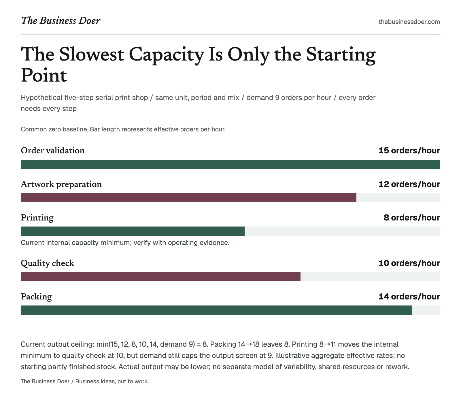
Visual reference. Current output ceiling: min(15, 12, 8, 10, 14, demand 9) = 8. Packing 14→18 leaves 8. Printing 8→11 moves the internal minimum to quality check at 10, but demand still caps the output screen at 9. Illustrative aggregate effective rates; no starting partly finished stock. Actual output may be lower; no separate model of variability, shared resources or rework.
Text version
Hypothetical five-step serial print shop / same unit, period and mix / demand 9 orders per hour / every order needs every step
- Order validation
- 15 orders/hour
- Artwork preparation
- 12 orders/hour
- Printing
- 8 orders/hour. Current internal capacity minimum; verify with operating evidence.
- Quality check
- 10 orders/hour
- Packing
- 14 orders/hour
Why does it matter?
Making an already fast step faster can improve its local metric without raising total output. It may simply create more work waiting for the next step.
Bottleneck analysis directs attention toward the restriction that matters for the whole workflow. It helps frame a staffing or equipment decision, investigate recurring delays and check whether an improvement has moved the limiting step elsewhere.
How bottleneck analysis works
Define the process and unit of work
Choose a clear start and finish. Define what moves through the process: an order, repair, application or customer request. A SIPOC diagram can establish the high-level boundary before detailed measurement.
Be specific about the mix. Ten simple print orders are not equivalent to ten complex jobs. If work varies substantially, separate meaningful groups or use an appropriate common workload measure before comparing capacities.
Measure each step’s effective capacity
Use the same unit and period for every step. For one resource processing one unit at a time:
Capacity = available processing time ÷ processing time per unit.
With 60 productive minutes and 6 minutes per comparable order, the simple rate is 10 orders per hour. If only 48 minutes are actually available, the same task supports 8 per hour. Establish which time basis you are using.
Record normal setup losses, downtime, rework, staffing and quality requirements where they affect the estimate. Do not subtract a loss again if the measured rate already includes it. The worksheet accepts comparable effective capacity rates; it does not calculate all these losses separately.
Compare capacity, demand and flow evidence
The lowest-capacity required step is the first candidate to investigate. Compare it with demand, then observe queues, actual completions, lost time and downstream waiting over a defined period.
A queue alone is not proof. Batching, temporary disruption, a missing approval or a different product mix can create one. High utilization also needs context: a busy machine producing the wrong work may not explain the customer’s delay.
Test an improvement and measure again
Investigate lost time, rework, handoffs, staffing or additional capacity at the candidate step. Preserve safety, required maintenance and quality.
Measure the whole process after the change, not just that step’s activity. A new internal minimum may emerge, or demand may become the tighter limit. Use a PDCA cycle to structure a small test before making a major commitment.
A worked example: five steps in a print shop
Hypothetical example. A small custom-print shop handles comparable orders through five required serial steps. Demand is 9 orders per hour. The figures below are invented teaching inputs, not observed performance or industry benchmarks.

Illustrative custom-printing workshop. The scene does not document the example's capacities or the results of a real business.
| Required step | Effective capacity, orders/hour |
|---|---|
| Order validation | 15 |
| Artwork preparation | 12 |
| Printing | 8 |
| Quality check | 10 |
| Packing | 14 |
Assume the same output unit, working period and mix; every order needs every step; there is no starting stock of partly finished orders. These aggregate rates already represent the assumed operating availability. Shared-resource conflicts, random variation, defects and rework are not modeled separately.
Printing is the internal capacity minimum at 8 orders/hour. Under this simple model:
Demand-limited output ceiling = min(15, 12, 8, 10, 14, demand 9) = 8 orders/hour.
If 9 orders continue arriving and printing consistently completes 8, with no cancellations, diversions or other changes, roughly one additional order per hour remains waiting to pass printing. That is a conditional flow imbalance, not a prediction of actual queue length or waiting time.
Improving the wrong step changes little
Suppose packing improves from 14 to 18 orders/hour. Printing still supports only 8. The internal capacity minimum and the demand-limited ceiling both remain 8 orders/hour.
The packing change could have other benefits, but it does not raise this model’s end-to-end throughput ceiling.
Improving printing moves the internal minimum
Now suppose reducing setup losses raises printing capacity from 8 to 11. The new internal capacity minimum is quality check at 10 orders/hour.
However, demand is still only 9. The output screen becomes:
min(15, 12, 11, 10, 14, demand 9) = 9 orders/hour.
The process capacity ceiling rises from 8 to 10, while the demand-limited output ceiling rises from 8 to 9. Neither number guarantees actual production, extra sales or profit. Quality check is the next internal capacity candidate, but demand is tighter under the current assumptions.
If demand later rises to 12 with the improved capacities unchanged, quality check would set the simple output ceiling at 10. Always state which demand and capacity assumptions support the conclusion.
When should you use it?
Use bottleneck analysis when work repeatedly queues, lead times increase, demand grows, teams are busy without more completions, or you are considering extra staff or equipment.
Do not assume every delay is a capacity problem. If the actual concern is an unverified defect, unclear demand, a policy or an external approval, investigate it rather than forcing it into a simple production-rate model.
How should you interpret the result?
A useful first diagnosis answers three questions:
- Where is the candidate capacity restriction?
- What operating evidence connects it to total flow?
- Would changing it improve the outcome that matters, given demand and other limits?
The Theory of Constraints is broader than this identification exercise: it also guides how to use the constraint well, align other work around it, increase capability when necessary and repeat. A company with spare production capacity can still be constrained by demand, approvals, cash or skills.
After a capacity restriction is verified, a fishbone diagram can organize possible causes of underperformance. The diagram does not itself prove the causes or identify the bottleneck.
Bottleneck versus the longest task
Task duration alone can be misleading. A 10-minute task with three genuinely independent, fully available parallel resources has a simple combined capacity of 18 units/hour. A 6-minute task with one such resource supports only 10.
That comparison assumes comparable work and no shared limiting resource. The worksheet requires each step’s aggregate effective capacity, not a single worker’s task time. Do not sum resources that compete for the same machine, approvals or materials as if they were independent.
Common mistakes and limitations
- Improving a non-limiting step and expecting total output to rise.
- Treating theoretical maximum speed as effective capacity.
- Ignoring demand or confusing a capacity ceiling with measured throughput.
- Treating a queue or a busy team as proof without checking the flow.
- Assuming the bottleneck cannot move, or overlooking tied minima.
- Increasing speed while damaging quality, maintenance or safe working conditions.
Real workflows can have variable arrivals, different routes, batching, shared resources and changing mix. The simple minimum rule is a screen for comparable serial steps, not a queueing simulation, staffing optimizer or causal diagnosis. In particular, it does not calculate waiting times. Use observation and a suitable process model before a major investment.
Put it to work: a 25-minute bottleneck scan
Choose one recurring workflow with three to six required steps. Define the boundary, output unit, period and mix. Record demand, each step’s realistic aggregate capacity, and what has actually been observed about queues, lost time or downstream waiting. Mark estimates and missing measurements honestly.
Compare the internal minimum with demand. Then test one hypothetical capacity change, holding the other inputs fixed. Finish with one improvement hypothesis, a whole-process outcome measure, quality/safety guardrails and a review point. The useful output is a candidate plus a measurement plan, not permission to buy equipment.
Use comparable output across a single serial route. All steps must handle the same unit, period and product mix. Decimal values are capacity rates, not partial completed orders.
- Name step 1.
- Step 1: Enter a capacity or demand amount.
- Name step 2.
- Step 2: Enter a capacity or demand amount.
- Name step 3.
- Step 3: Enter a capacity or demand amount.
- Demand: Enter a capacity or demand amount.
- Record the common output unit and period.
- Confirm comparable serial capacities and the model assumptions before calculating.
- Process boundary: record the evidence or what is missing.
- Demand evidence: record the evidence or what is missing.
- Observation context and capacity basis: record the evidence or what is missing.
- Step 1 evidence / flow observation: record the evidence or what is missing.
- Step 2 evidence / flow observation: record the evidence or what is missing.
- Step 3 evidence / flow observation: record the evidence or what is missing.
- Improvement hypothesis
- Whole-process measure and guardrails
- Review point and owner
Quick checklist
Final takeaway
Find the restriction that limits the whole workflow, not simply the task that looks slowest. Compare effective capacities consistently, check demand and verify the candidate against operating evidence.
Then test a focused change and measure again. Improving one step can move the internal minimum without making it the business’s active constraint.